Is Climate Change Real — And Why Should We Care?

Old Man Rainforest Eating His Daily Red Beans

A Jellybean Jar, a Pile of Nuclear Reactors, and a Few Rainforests

I’ve always believed in science. But as an engineer, I like to stress-test assumptions. One question nagged at me: if Earth was warmer in the age of the dinosaurs, why should we believe today’s warming is different, or that it’s caused by us? I turned to the record—satellites watching Earth’s glow, ships and floats measuring the oceans, ice cores drilled from two miles down—and I asked for everything in plain numbers: watts, joules, and parts per million. I wanted units a curious kid or a tough-minded engineer could track across a dinner table.

What came back wasn’t subtle. Yes, Earth has been hotter. What’s different now is the speed. Nature’s thermostat drifts in slow motion; ours is a hand on the dial. To make the story concrete, I compressed centuries of climate physics into three pictures: jellybeans for greenhouse gases, nuclear reactors for continuous trapped heat, and a rainforest ledger for the give-and-take between emissions and the planet’s natural sinks.

Background: When Science First Figured It Out

• 1824 — Joseph Fourier noticed Earth was too warm for its distance from the Sun. He proposed that the atmosphere acts like a blanket, trapping heat (Fourier, 1824).

• 1859 — John Tyndall proved in the lab that gases like CO₂ and water vapor absorb infrared radiation, showing how the blanket works (Tyndall, 1861).

• 1896 — Svante Arrhenius did the first calculation linking fossil fuels to global warming. His pencil-and-paper math suggested that doubling CO₂ would warm Earth by ~5–6 °C (Arrhenius, 1896). Modern models say ~3 °C. Not bad for the 19th century.

• 1938 — Guy Callendar compiled weather records and showed that global temperatures were already rising, consistent with coal burning (Callendar, 1938).

• 1958 — Charles Keeling began precise CO₂ measurements at Mauna Loa, Hawaii, producing the iconic “Keeling Curve” (Keeling, 1960).

• 1979 — The Charney Report from the U.S. National Academy of Sciences concluded: doubling CO₂ would warm Earth by 1.5–4.5 °C. That’s still the range we cite today (Charney et al., 1979).

The physics is old. The evidence is long-standing. And the predictions have held up for more than a century.

Now, let’s make the science tangible—with jellybeans, nuclear reactors, and rainforests.

The Jellybean Jar

Picture the atmosphere as a jar with a million jellybeans. Most beans are harmless nitrogen and oxygen. The “special red beans” are the heat-trapping gases. Before factories and steam engines, there were about 278 red beans in the jar—278 ppm CO₂-equivalent (ppm CO₂e). Today there are roughly 534 ppm CO₂e. Every year we add about 3 ppm CO₂e. That sounds tiny until you remember the last deglaciation added only ~80 ppm CO₂e in ~6,000 years—about 0.013 ppm CO₂e per year. We’re now adding beans to the jar nearly 250× faster than that long, gentle rise.

Fact Check

• Pre-industrial CO₂e ≈ 278 ppm: Ice core records show atmospheric CO₂ around 278 parts per million before 1750 (Petit et al., 1999).

• Today ≈ 534 ppm CO₂e: NOAA’s Annual Greenhouse Gas Index (AGGI) reports a combined CO₂-equivalent concentration of ~534 ppm in 2023 (NOAA, 2024).

• Current growth ≈ +3 ppm per year: Long-term monitoring at Mauna Loa and global networks find CO₂ increasing by ~2.5–3.0 ppm annually (NOAA, 2024).

• Last deglaciation ≈ +80 ppm over 6,000 years: Ice core data show CO₂ rising from ~190 ppm to ~270 ppm at the end of the last Ice Age, a rate of ~0.013 ppm per year (Petit et al., 1999).

• Today’s pace ≈ 250× faster: Comparing today’s ~3 ppm per year to the deglacial ~0.013 ppm per year shows the modern rise is ~230–250 times faster (Petit et al., 1999; NOAA, 2024). 

Reactors in the Ocean

Each extra bean tweaks the planet’s energy balance. Scientists call the nudge radiative forcing and measure it in watts per square meter (W/m²). The human-added beans since 1750 now trap about 3.49 W/m². Spread across Earth’s area (510 million km²), that’s roughly 1,780 terawatts (TW) of continuous heating. In human terms, that’s the heat of ~460,000 large nuclear reactors running 24/7, invisible, whose sole purpose is warming the ocean. This assumes the electricity from those reactors is also converted into heat by sinking the current into resistors under the ocean.  And the dial is still turning: forcing is rising by ~0.036–0.037 W/m² each year, another ~18 TW, or about 4,000 new reactor equivalents per year.

Fact Check

• Radiative forcing ≈ 3.49 W/m²: NOAA’s Annual Greenhouse Gas Index (AGGI) estimates that human-added greenhouse gases since 1750 trap ~3.49 watts per square meter of extra energy (NOAA, 2024).

• Earth’s surface area ≈ 510 million km²: The U.S. Geological Survey reports Earth’s area as ~5.10 × 10¹⁴ m² (USGS, 2012). Multiplying by 3.49 W/m² gives ~1.78 × 10¹⁵ W, or 1,780 terawatts.

• Reactor equivalents ≈ 460,000: A modern European Pressurized Reactor (EPR) produces ~4.59 gigawatts thermal (World Nuclear Association, 2025). Dividing 1,780 TW by 4.59 GW yields ~460,000 reactors.

• Annual increase ≈ 0.036–0.037 W/m²: The NOAA AGGI trend line shows forcing rising by ~0.037 W/m² per year (NOAA, 2024).

• Extra heating ≈ 18 TW/year: Multiplying 0.037 W/m² by Earth’s area gives ~1.88 × 10¹³ W, or ~18 TW of additional heating each year.

• Equivalent to ~4,000 new reactors annually: Divide 18 TW by 4.59 GW per reactor, and you get ~4,000 more reactors’ worth of heat every year (World Nuclear Association, 2025).

Paris drew the lines. The data show where we really are.

The 2015 Paris Agreement asked the world to keep warming “well below 2 °C,” ideally 1.5 °C. Those targets are temperature outcomes. The physics links them to forcing thresholds. In forcing terms, the world crossed the 1.5 °C-equivalent (steady state equivalent) back in the early 1980s and the 2.0 °C-equivalent by the late 1990s. That can be unsettling until you remember the ocean is a slow giant: it soaks up heat and delays the full surface response. Inertia is not mercy; it’s latency. So, at the time the Paris Agreement was signed those temperature increases had not manifested yet. 

Fact Check

• Paris Agreement targets: In 2015, nearly every country pledged to keep warming “well below 2 °C” and pursue efforts toward 1.5 °C (UNEP, 2023). These limits are defined in surface temperature change (°C).

• Link to forcing thresholds: Climate physics connects greenhouse gas concentrations to radiative forcing using the logarithmic formula RF = 5.35 × ln(C/C0) (Myhre et al., 1998). At equilibrium, warming is RF ÷ λ, where λ ≈ 1.233 W/m² per °C (IPCC, 2021).

• Crossing 1.5 °C-equivalent: NOAA’s AGGI series shows effective radiative forcing exceeded the 1.5 °C equilibrium threshold (~1.88 W/m²) by the early 1980s (NOAA, 2024).

• Crossing 2.0 °C-equivalent: The 2.0 °C threshold (~2.5 W/m²) was passed in the late 1990s (NOAA, 2024).

• Why temperatures lag: The ocean’s vast heat capacity absorbs most of the extra energy, delaying the surface warming by decades to centuries (Hansen et al., 2011; Geoffroy et al., 2013). This “thermal inertia” explains why the Paris goals were already exceeded in forcing terms, but not yet in observed surface temperatures

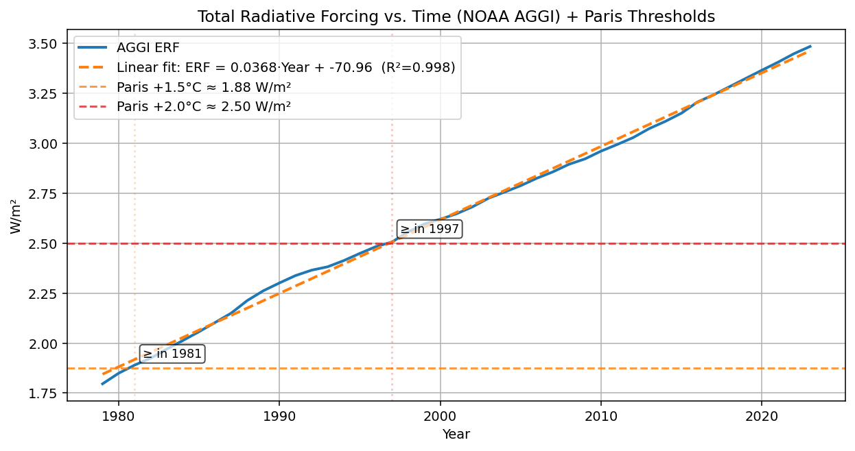
Figure 1: Total Radiative Forcing vs. Time (NOAA AGGI) + Paris Thresholds

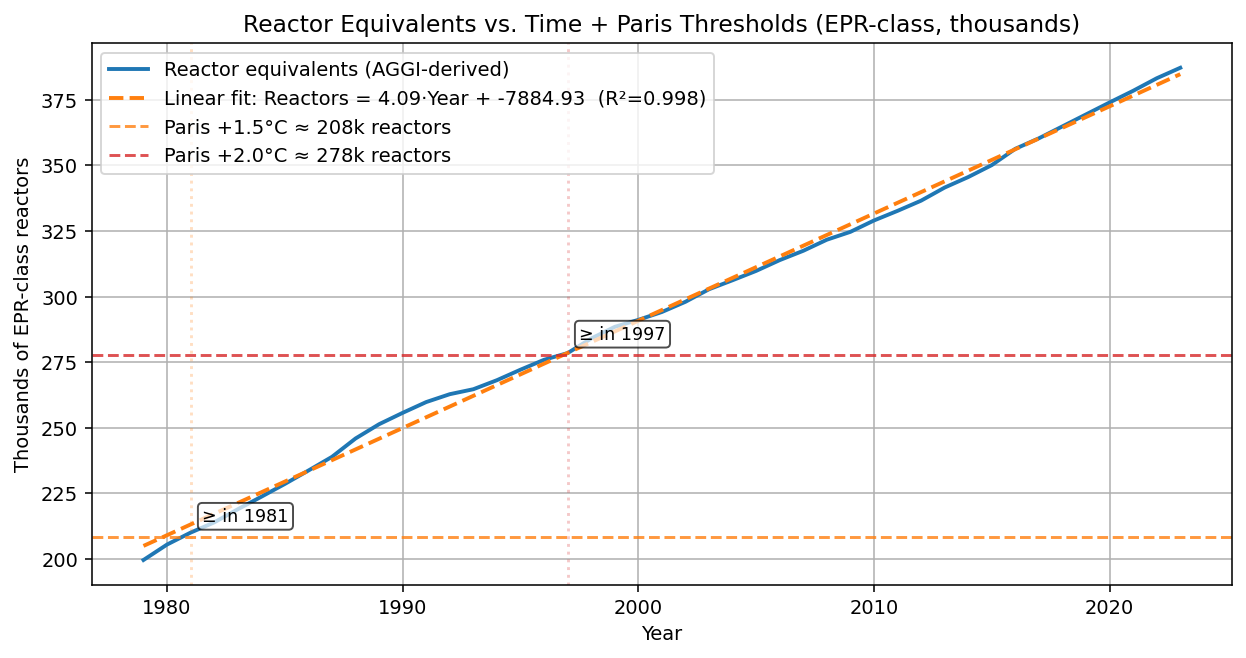
Figure 2: Reactor Equivalents vs. Time + Paris Thresholds (EPR-class)

Every extra jellybean doesn’t just sit in the jar — it adds heat. The physics is straightforward: radiative forcing grows with the natural logarithm of greenhouse gas concentration. That means each new ppm CO₂e adds a little less than the one before, but as long as we keep adding them quickly, the total “push” keeps climbing. The equation looks like this:

Radiative forcing (RF) = 5.35 × ln(C / C0)

·       RF is the imbalance at the top of the atmosphere, in watts per square meter (W/m²).

·       C is today’s greenhouse gas concentration in ppm CO₂e (all gases converted to CO₂-equivalent).

·       C0 is the pre-industrial baseline of 278 ppm CO₂e.

Plug in today’s numbers, and we get an RF of about 3.49 W/m². Multiply by Earth’s surface area (5.1 × 10¹⁴ m²), and that’s 1,780 trillion watts of excess heating. To make that tangible, divide by the thermal output of a European Pressurized Reactor (4.59 GWₜ), and you get the staggering picture (this is an analogy):

≈ 460,000 nuclear reactors’ worth of heat are already running full throttle in the oceans.

And it’s not static. Each year, forcing increases by ~0.036 W/m² — equivalent to 18 terawatts, or about 4000 new reactors added annually. Imagine secretly building thousands of massive nuclear plants under the sea every year, all designed not to produce electricity, but just to warm the planet. That is effectively what fossil fuels are doing.

These two figures tell the same story in two different languages. The first shows effective radiative forcing in W/m², with a nearly perfect straight-line trend (R² ≈ 0.998). The second translates that same heat into “reactor equivalents,” a rising stack of imaginary power stations humming away beneath the waves. Either way you look at it, the trajectory is astonishingly straight — and astonishingly steep.  This is surprising, because Radiative Forcing goes as the natural logarithm of CO2e, but wait, does that mean CO2e is going up exponentially to make Radiative Forcing go up linearly?

Fact Check

• Forcing formula: The standard expression for greenhouse gas forcing is RF = 5.35 × ln(C / C0), where RF is radiative forcing in watts per square meter (W/m²), C is current greenhouse gas concentration in ppm CO₂-equivalent (CO₂e), and C0 is the pre-industrial baseline of 278 ppm CO₂e (Myhre et al., 1998; IPCC, 2021).

• Today’s forcing: Plugging in today’s concentration (~534 ppm CO₂e) gives RF ≈ 3.49 W/m², consistent with NOAA’s Annual Greenhouse Gas Index (NOAA, 2024).

• Total heating power: Multiplying by Earth’s surface area (5.1 × 10¹⁴ m²; USGS, 2012) yields ~1.78 × 10¹⁵ W, or 1,780 terawatts (TW) of continuous heating.

• Reactor equivalents: Dividing by the thermal output of an EPR-class reactor (~4.59 GWₜ; World Nuclear Association, 2025) gives the striking analogy of ~460,000 reactors’ worth of heat already operating full time in the oceans.

• Annual increase: Radiative forcing has been rising at ~0.036–0.037 W/m² per year since the late 1970s, equivalent to ~18 TW per year, or about 4,000 new reactor equivalents annually (NOAA, 2024).

• Why linear forcing? Radiative forcing increases logarithmically with CO₂e, so a perfectly linear rise in forcing implies that CO₂e concentration itself has been increasing nearly exponentially. This pattern has indeed been observed in recent decades (NOAA, 2024).

Beans to Forcing to Heat: a single curve

Because forcing grows logarithmically with greenhouse gases, each new jellybean (each extra ppm CO₂e) adds a little less push than the previous one. But if we keep tossing beans in faster and faster, the total push still climbs steadily. The relationship scientists use (Myhre et al., 1998) is:

Radiative forcing (RF) = 5.35 × ln(C / C0) [units: W/m²]

·       RF is the extra heat “push” on the climate system, in watts per square meter (W/m²).

·       5.35 is an empirical constant that links concentration to forcing. Its units are W/m² per unit of natural log.

·       ln(… ) is the natural logarithm.

·       C is the current concentration of greenhouse gases in the air, measured here as CO₂-equivalent (ppm CO₂e) so that CO₂, methane, nitrous oxide, etc., all live in the same currency.

·       C0 is the pre-industrial baseline, taken as 278 ppm CO₂e.

Two immediate takeaways:

1.     If you double C (so C/C0 = 2), then ln(2) ≈ 0.693 and RF ≈ 5.35 × 0.693 ≈ 3.7 W/m². That’s why “a doubling of CO₂” (relative to pre-industrial levels) is often linked to ~3.7 W/m² of forcing.

2.     The log means the first 100 ppm added more forcing than the next 100 ppm—but as long as C keeps climbing, RF keeps rising.

To turn forcing into something you can feel, multiply RF by Earth’s surface area to get power:

Planetary heating (Watts) = RF × Earth area
Earth area ≈ 5.10 × 10¹⁴ m², so 1 W/m² ≈ 510 terawatts (TW) of extra heating.

Then translate that heat into “reactor equivalents”; let’s look at that math more closely:

Reactor equivalents = (RF × Earth area) / (total reactor thermal power)
Using an EPR-class reactor at about 4.59 gigawatts thermal (GWₜ), today’s RF (~3.49 W/m²) corresponds to roughly 460,000 reactors running nonstop.

Now map ppm CO₂e → RF → reactor equivalents, and you get the curve below. Put three flags on it—2100, 2200, and 2300—and “business as usual” stops being abstract. Each waypoint is just a different C in the same equation, converted to W/m², then to TW, then to a stack of imaginary reactors humming under the waves.  This assumes radiative forcing continues on the same linear trajectory, then CO2e is calculated from the projected radiative forcing. 

Fact Check

• Forcing relationship: The formula RF = 5.35 × ln(C / C0) is the standard expression for radiative forcing of well-mixed greenhouse gases, where C is the present concentration in ppm CO₂-equivalent and C0 is the pre-industrial baseline of 278 ppm (Myhre, Highwood, Shine, & Stordal, 1998; IPCC, 2021).

• Doubling CO₂ → 3.7 W/m²: Setting C/C0 = 2 gives ln(2) ≈ 0.693, and RF ≈ 3.7 W/m², which is the canonical forcing associated with a CO₂ doubling (IPCC, 2021).

• Uneven forcing per 100 ppm: Because the formula is logarithmic, the first 100 ppm added more forcing than the next 100 ppm, but as long as concentration keeps rising, forcing continues to climb.

• Earth’s area → power: Earth’s surface area is ~5.10 × 10¹⁴ m² (USGS, 2012). Multiplying RF (W/m²) by this area converts forcing into total planetary heating in watts. For example, 1 W/m² corresponds to ~510 terawatts (TW).

• Today’s forcing → ~460,000 reactors: With RF ≈ 3.49 W/m² (NOAA, 2024), total heating is ~1.78 × 10¹⁵ W. Dividing by the thermal output of an EPR-class reactor (~4.59 GWₜ; World Nuclear Association, 2025) gives ~460,000 reactors’ worth of heat.

• Business-as-usual mapping: If forcing continues its observed linear climb (~0.037 W/m² per year; NOAA, 2024), then future ppm CO₂e can be back-calculated from projected forcing using the same logarithmic relationship. This lets us place waypoints for 2100, 2200, and 2300 on the “ppm → forcing → TW → reactors” curve.

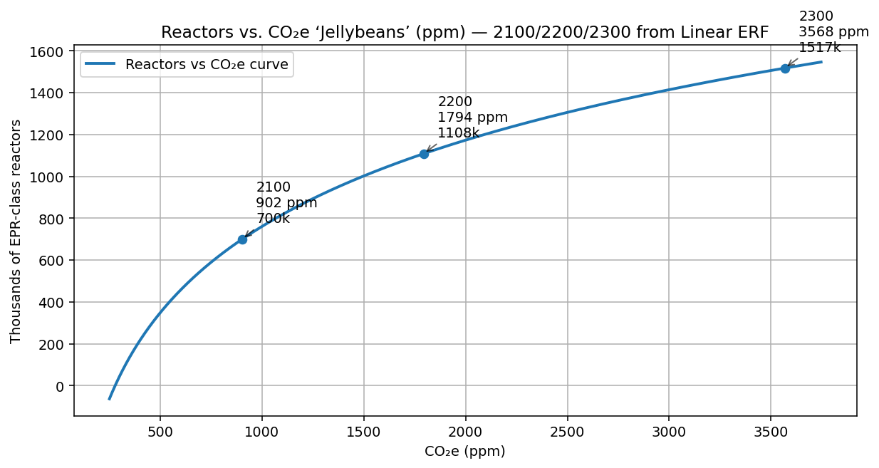
Figure 3: Reactors vs. CO₂e (“Jellybeans”) — 2100/2200/2300 from Linear ERF

The markers show one possible pathway if today’s nearly linear forcing growth continues: passing ~900 ppm CO₂e by 2100, ~1,800 ppm CO₂e by 2200, and >3,500 ppm CO₂e by 2300. That last number lives in deep geologic time.

How confident are we in the linear trend? The residuals tell the tale.  At least over the last 45 years, the residuals on the linear radiative forcing curve are < +/- 0.05 W/m2. 

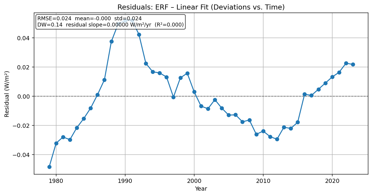
Figure 4: Residuals — ERF minus Linear Fit (Deviations vs. Time)

The dots hug zero with a root-mean-square wiggle of only a few hundredths of a watt per square meter. For the next few decades, a straightedge is a reasonable guide. By the far future, additional feedbacks—melting ice, shifting clouds, thawing permafrost—could bend the line. Changes in human behavior is also a big question mark.  How seriously will we take this problem?  But the near-term message is simple: we are still climbing.

Fact Check

• Projected concentrations: If radiative forcing continues its observed near-linear climb (~0.037 W/m² per year; NOAA, 2024), the implied CO₂-equivalent (CO₂e) concentrations would be ~900 ppm by 2100, ~1,800 ppm by 2200, and >3,500 ppm by 2300. Such values are comparable only to levels seen tens of millions of years ago in Earth’s geologic past (Foster, Royer, & Lunt, 2017).

• Residuals check linearity: The NOAA AGGI dataset fits a straight line with R² ≈ 0.998, and the residuals remain within ±0.05 W/m² over the past 45 years. The root-mean-square error (RMSE) is only ~0.024 W/m², meaning deviations are tiny compared to the overall rise (NOAA, 2024).

• What it means: In the near term, a straightedge is a reasonable guide for forcing growth. However, over centuries, additional climate feedbacks—melting ice, changes in cloud cover, thawing permafrost—could bend the trajectory (IPCC, 2021). Human decisions about emissions will also strongly influence whether the straight line continues.

The Rainforest Ledger

Think of the atmosphere as a ledger. On the deposit side, humanity currently emits about 57 billion tonnes CO₂e per year, which is ~7.3 ppm CO₂e per year added to the jar. On the withdrawal side, oceans, forests, and soils pull down ~4.2 ppm CO₂e per year. The remainder—~3.1 ppm CO₂e per year—stays in the air. The Amazon rainforest, when healthy, removes roughly 1.6 billion tonnes CO₂ per year, or ~0.2 ppm CO₂e per year. That means it takes five Amazons to erase a single bean from the ledger each year. To cancel the leftover 3.1 ppm CO₂e we’d need ~15 totally new Amazons. Then, we’d be breaking even on the jelly bean jar. This tells a stark picture, because planting 15 new Amazon rainforests would be quite a challenging problem.  We have one Amazon—and parts of it, scarred by deforestation and heat, are now a source rather than a sink.  In fact, all around the world deforestation is a major problem. 

Fact Check

• Emissions today: Humanity emits ~57 gigatonnes of CO₂-equivalent (GtCO₂e) annually, adding about 7.3 ppm CO₂e per year to the atmosphere (UNEP, 2023; NOAA, 2024).

• Natural sinks: Oceans, forests, and soils collectively absorb about 4.2 ppm CO₂e per year, leaving a net gain of ~3.1 ppm CO₂e per year in the air (Friedlingstein et al., 2020; NOAA, 2024).

• Amazon’s role: The intact Amazon rainforest removes about 1.6 GtCO₂ per year, equivalent to ~0.2 ppm CO₂e per year (Hubau et al., 2020).

• Scaling the math: It would take five Amazons to remove one ppm CO₂e per year, and ~15 Amazons to cancel today’s leftover growth of 3.1 ppm CO₂e annually.

• Limits of the ledger: We have only one Amazon, and research shows parts of it have already flipped to being a net carbon source due to deforestation, drought, and warming (Gatti et al., 2021). Globally, deforestation continues to weaken the land sink (IPCC, 2021).

If we keep going

What would the world feel like if the straight line from Figure 1 keeps running? With a constant climb of about 0.0368 W/m² per year (the slope of the regression line, R² ≈ 0.998), forcing would rise to around 13.7 W/m² by 2300. The equilibrium warming linked to that level of forcing is about 11.1 °C above pre-industrial, using the standard climate feedback parameter (λ ≈ 1.233 W/m² per °C, equivalent to 3 °C per CO₂ doubling). Because the oceans act as a massive heat sink and slow the adjustment, the realized surface warming in 2300 would still reach roughly 8.6 °C—about four times today’s warming—even as the higher equilibrium keeps tugging upward for centuries after.

At those temperatures, the phrase “different planet” stops being metaphor. The Arctic likely loses its summer sea ice this century near ~2 °C. Greenland commits to large-scale melt beyond ~3 °C; Antarctica destabilizes somewhere past ~4–6 °C. At >10 °C, both poles eventually head for an ice-free state reminiscent of warm deep-time climates. Sea level rise becomes a matter not of centimeters or even a single meter, but the tens of meters—~60–70 m if Greenland and Antarctica fully melt—unfolding over centuries to millennia. Every coastal city goes under. Deltas that feed hundreds of millions—Nile, Mekong, Ganges-Brahmaputra—shrink or drown. Hotter oceans and moister air supercharge storms and floods; hotter land stretches droughts and fires. In parts of South Asia and the Middle East, “wet-bulb” heat pushes past human survivability without active cooling.

That is the straight-line future. It is not destiny. It is the future that happens if we don’t turn.

Fact Check

• Regression slope: NOAA’s Annual Greenhouse Gas Index shows effective radiative forcing has increased almost linearly since 1979, at ~0.0368 W/m² per year, with R² ≈ 0.998 (NOAA, 2024).

• Forcing by 2300: Extrapolating that slope implies forcing of ~13.7 W/m² by 2300.

• Equilibrium warming: Using λ ≈ 1.233 W/m² per °C (climate feedback parameter consistent with ~3 °C per CO₂ doubling), equilibrium warming at 13.7 W/m² forcing is ~11.1 °C above pre-industrial (IPCC, 2021; Myhre et al., 1998).

• Realized surface warming: A two-box energy balance model (surface + deep ocean) suggests ~8.6 °C realized warming by 2300, since ocean heat uptake delays the full adjustment (Geoffroy et al., 2013).

• Cryosphere thresholds:

• Arctic summer sea ice is projected to vanish near 2 °C warming (IPCC, 2021).

• Greenland commits to large-scale melt beyond ~3 °C (Clark et al., 2016).

• Antarctica destabilizes somewhere past ~4–6 °C (IPCC, 2021).

• Sea level rise: A complete melt of Greenland and Antarctica would eventually raise seas by ~60–70 meters, though over centuries to millennia (Clark et al., 2016; IMBIE Team, 2018).

• Extreme impacts: At >10 °C warming, habitability shrinks dramatically: river deltas drown, extreme storms intensify, droughts and wildfires expand, and “wet-bulb” heat in South Asia and the Middle East exceeds human survivability thresholds (Sherwood & Huber, 2010; Pal & Eltahir, 2016).

Deep Dive (for the curious): the system underneath the story

If you like to see the gears turning, here an even deeper dive into the system dynamics of earth’s climate change.  Below is a bond graph, which is a type of model for dynamic systems used by systems engineers. 

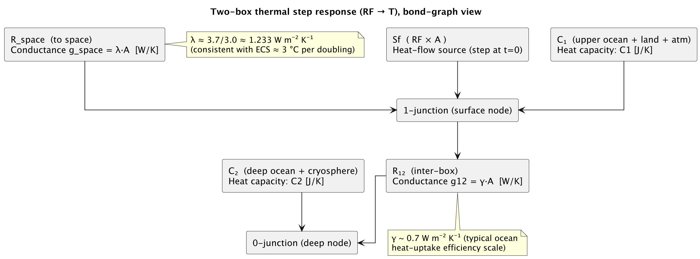
Figure 5: Two-Box Thermal Step Response — Bond-Graph View

When engineers and physicists want to understand how energy moves, they often draw something called a bond graph. It’s a kind of map that shows where energy is stored, where it flows, and where it leaks away. In our climate sketch, the heat source is the radiative forcing (the extra watts per square meter trapped by greenhouse gases) multiplied by Earth’s surface area. That’s the faucet pouring energy into the system.

The first reservoir is the surface layer — the atmosphere, the land, and the upper ocean — with a heat capacity we call C1, measured in joules per degree (J/K). The second reservoir is the deep ocean and ice, with an even larger heat capacity C2. Think of them as two buckets of water stacked on top of each other: the top bucket – which has a smaller capacity – warms quickly, while the bottom one takes centuries to catch up.

Energy leaks to space through a conductance called g_space, measured in watts per degree (W/K). This is defined by a parameter called lambda (λ), the climate feedback strength, which tells us how strongly Earth radiates heat back to space as it warms. Based on decades of science, λ is about 1.233 W/m² per °C, which comes from the classic result that doubling CO₂ (adding about 3.7 W/m² of forcing) warms Earth roughly 3 °C at equilibrium (Myhre et al., 1998; IPCC, 2021). There’s also a second conductance, g12, that represents how efficiently the surface passes heat down to the deep ocean. A typical value is about 0.7 W/m² per °C (Geoffroy et al., 2013).

These pieces come together at special “junctions.” The surface junction balances energy flows, while the deep junction shares a common temperature. With two independent energy stores, the system naturally develops two time scales: a fast adjustment (years to decades) as the surface warms, and a slow adjustment (centuries) as the deep ocean and ice absorb heat. In control systems language, that means Earth’s temperature response is at least a two-pole transfer function — not a simple one-knob thermostat.

Written out in plain text, the equations look like this:

• Surface: C1 × dT1/dt = RF(t) × Area − g_space × T1 − g12 × (T1 − T2)

• Deep: C2 × dT2/dt = g12 × (T1 − T2)

Here T1 is the surface warming (°C) above pre-industrial, and T2 is the deep ocean and ice warming. At steady state, both buckets eventually reach the same temperature, and the simple rule emerges: equilibrium warming = RF ÷ λ.

So what happens if we start with pre-industrial levels and then flip a switch to today’s forcing and just wait? Today’s forcing is about 3.49 W/m² (NOAA, 2024). Divide that by λ (1.233 W/m² per °C), and the equilibrium warming is about 2.83 °C above pre-industrial. In engineering language, that’s called a “step function”.  That isn’t what really happened because the radiative forcing didn’t jump to 460,000 nuclear reactor equivalents overnight.  But, the 2.83 °C is where the system wants to go in steady state. But because the deep ocean is such a massive heat sink, we don’t jump there right away. The surface warms quickly, then creeps upward for centuries as the deep ocean gradually fills with heat.

This is exactly what the “step response” figure shows. The blue curve (surface) rises fast at first, while the orange curve (deep ocean) lags behind. Both are heading toward the dashed line at 2.83 °C, but it takes centuries to get there. In other words: even if we froze greenhouse gases at today’s levels, Earth would still have a couple degrees of warming “baked in,” waiting to unfold as the deep ocean catches up.

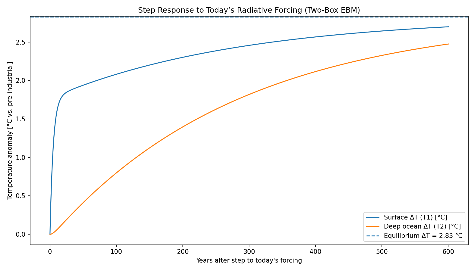
Figure 6: Step Response to Today’s Forcing (Two-Box Energy Balance Model)

Freezing today’s forcing (~3.49 W/m²) leaves the system aiming for an equilibrium of roughly 2.83 °C of warming relative to pre-industrial levels. The surface warms quickly at first, then crawls as the deep ocean continues to soak up heat for centuries.

Now let’s see what happens the forcing keep climbing along the observed straight line from Figure 1. 

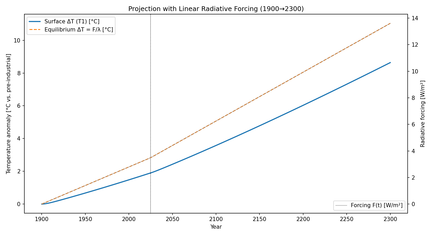
Figure 7: Projection with Linear Radiative Forcing (1900→2300)

From a 20th-century ramp to the present, then onward with ~0.037 W/m² per year, the realized surface temperature (solid line) rises toward the moving equilibrium line (dashed). By 2300, the model delivers the numbers used earlier: ~8.6 °C realized with ~11.5 °C equilibrium tugging above it.  The radiative forcing is shown on the 2nd Y-axis on the right and perfectly overlaps with the equilibrium change in temperature as expected. 

Fact Check

• Bond graphs: Engineers and physicists use bond graphs to represent how energy is stored, transferred, and dissipated. In climate EBMs, the heat source is radiative forcing (RF, W/m²) × Earth’s area (m²), feeding into reservoirs that represent the climate system (Karnopp, Margolis, & Rosenberg, 2012).

• Heat capacities:

• C1 (surface layer) covers the atmosphere, land, and upper ocean.

• C2 (deep layer) represents the deep ocean and cryosphere.
  Heat capacities are expressed in joules per kelvin (J/K) and determine how much warming occurs per unit of added energy (Geoffroy et al., 2013).

• Conductances:

• g_space = λ × A, where λ is the climate feedback parameter (about 1.233 W/m² per °C), reflecting how efficiently Earth radiates heat back to space as it warms. This λ is consistent with an equilibrium climate sensitivity (ECS) of ~3 °C per CO₂ doubling (Myhre et al., 1998; IPCC, 2021).

• g12 = γ × A, where γ ≈ 0.7 W/m² per °C, represents the exchange of heat between surface and deep ocean (Geoffroy et al., 2013).

• Two time scales: With two reservoirs, Earth has a fast timescale (years to decades, surface adjustment) and a slow timescale (centuries, deep ocean filling). This is why Earth’s climate acts like a two-pole transfer function, not a single thermostat.

• Step response math:

• Governing equations:
  • C1 × dT1/dt = RF × A − g_space × T1 − g12 × (T1 − T2)
  • C2 × dT2/dt = g12 × (T1 − T2)

• With today’s forcing of ~3.49 W/m² (NOAA, 2024) and λ = 1.233 W/m² per °C, equilibrium warming = RF ÷ λ ≈ 2.83 °C above pre-industrial.

• Why it matters: Even if forcing froze today, the step response shows Earth still has ~2–3 °C of warming “in the pipeline” as the deep ocean continues to absorb heat.

Final words (and a promise)

This essay has been about defining the problem. Along the way, we’ve walked through a set of analogies and models designed to make the invisible visible.

The jellybeans showed how greenhouse gases accumulate in the air, measured in parts per million of CO₂-equivalent (ppm CO₂e). What once looked like a handful of red beans has now grown into more than five hundred, with a few more being tossed in every single year.

The reactors translated those beans into heat — not an abstraction, but the steady hum of terawatts of energy. Today’s forcing is like secretly running almost half a million nuclear power plants beneath the waves. Each year adds another four thousand, built not to light homes or power cities, but solely to make the planet warmer.

The rainforest ledger showed the imbalance between deposits and withdrawals. Humanity adds about 57 billion tonnes of CO₂e per year, equivalent to more than seven beans. Nature withdraws about four of them, leaving three beans behind in the jar every year. The Amazon rainforest, even when intact, can only eat about a fifth of a bean. We would need fifteen Amazons just to break even, but instead we are weakening the only one we have.

The Paris Agreement thresholds gave us a sobering reality check. In terms of radiative forcing, we had already crossed the 1.5 °C equivalent in the early 1980s and the 2.0 °C equivalent by the late 1990s. The only reason the thermometer does not yet reflect those numbers is because the oceans and ice are buying us time, storing heat like giant flywheels. But stored heat is not spared heat. It still comes back to the surface.

The residuals plot told us the trend has been eerily straight. Since the late 1970s, effective radiative forcing has risen almost perfectly linearly, at about 0.037 W/m² per year. That straight line is the simplest guide to where we are headed if nothing changes.

The step response showed what happens if we froze today’s forcing in place. The system would aim for about 2.83 °C of warming above pre-industrial, with the surface racing upward at first, then slowing as the deep ocean filled. Even without another gram of CO₂, we still have more warming “in the pipeline.”

The energy balance model (EBM) explained why. With two reservoirs of heat — the surface and the deep — the climate system has two characteristic timescales. One is fast, measured in years to decades, as the surface warms. The other is slow, measured in centuries, as the deep ocean and ice absorb their share. Engineers call this a two-pole transfer function. In everyday terms, it’s why climate change feels slow even when it’s actually relentless. The EBM is not a crystal ball, but it distills two centuries of physics into equations simple enough to run on a laptop. It helps us see what’s already baked in, and why the Paris thresholds were never “lines in the sand” so much as “lines we crossed decades ago.”

Finally, the linear projection showed us business-as-usual. Carry the straight line forward, and by 2300 forcing rises to nearly 14 W/m². The equilibrium warming that corresponds to is about 11 °C, while the realized surface temperature is about 8.6 °C — four times the warming we’ve seen so far. That is a world transformed. Seas rise not by centimeters or even meters, but by tens of meters as Greenland and Antarctica melt. Every coastal city drowns. Croplands shift. Storms intensify. Regions of South Asia and the Middle East face wet-bulb conditions beyond human survivability. The poles head toward a state not seen for more than 30 million years: ice-free.

This essay has been about the problem statement and the context: what the numbers mean, what the trends look like, and why the physics is unyielding. It can feel grim, but clarity is not the same as despair. Problems exist to be solved, and the path is still ours to choose.

The next posts will shift from the problem to the solutions: scaling renewable energy, electrifying everything from cars to steel mills, redesigning cities and industries, restoring forests and ecosystems, pulling carbon back out of the air, and changing daily habits like moving toward plant-based diets that cut emissions without lowering quality of life.

The straight line only continues if we let it. The question is no longer whether the problem is real. It is whether we choose to bend that line, together.

Climate Change Q&A

Common Questions, Some for Skeptics, & Evidence-Based Answers

Q1. Isn’t climate always changing? Why should we care if it’s warming now?
A. Yes, Earth’s climate has changed many times due to natural cycles. What’s different today is the speed and cause. We’re adding greenhouse gases ~250× faster than the natural deglaciation rate. Past shifts took thousands of years; today’s is happening in decades (Petit et al., 1999; NOAA, 2024).

Q2. Aren’t most temperature sensors in big cities, making them unreliable because of the “urban heat island” effect?
A. Scientists correct for urban heat islands. Global warming is confirmed by satellites, ocean buoys, rural stations, and ice cores. All show the same warming trend (Hansen et al., 2010; Roemmich et al., 2019; Santer et al., 2013).

Q3. Don’t satellites actually measure Earth’s radiation balance? Isn’t that the best evidence?
A. Exactly. Earth is monitored like an optical power balance: instruments like CERES measure reflected shortwave sunlight and outgoing infrared, while SORCE and TSIS measure incoming solar irradiance. The imbalance is Earth’s radiative forcing. Satellites consistently show Earth is retaining about 0.9 W/m² more than it emits, confirmed by ocean heat uptake (Loeb et al., 2012; Kopp & Lean, 2011; NASA, 2023).

Q4. CO₂ is just a trace gas—less than 0.1% of the atmosphere. How can it matter?
A. Small amounts can have big effects. The ozone layer is only a few parts per million yet shields all life from UV. CO₂ is a trace gas, but it controls Earth’s heat balance. Without it, Earth would be frozen (Arrhenius, 1896; IPCC, 2021).

Q5. Didn’t Earth used to be warmer, like during the dinosaur age?
A. Yes, but human civilization developed in the stable climate of the last ~10,000 years. Today’s rapid warming threatens food, infrastructure, and ecosystems humans depend on (Foster et al., 2017; Clark et al., 2016).

Q6. What about natural causes—like the sun or volcanoes?
A. Solar output has been flat or slightly down since the 1970s, while temperatures rose sharply. Volcanoes cause temporary cooling. Only greenhouse gases match the observed warming (Lean & Rind, 2008; Kopp & Lean, 2011).

Q7. Haven’t climate models been wrong before?
A. Models aren’t perfect, but they’ve been very accurate over decades. Predictions from the 1980s align well with observed warming. The uncertainty is in our choices about emissions, not in the physics (Hausfather et al., 2020; IPCC, 2021).

Q8. Isn’t CO₂ good for plants?
A. CO₂ can boost plant growth in greenhouses, but in the real world heatwaves, droughts, and fires cause far more harm. Food security declines under higher warming (Zhao et al., 2017; Hubau et al., 2020).

Q9. Haven’t past predictions of catastrophe been exaggerated?
A. Scientists don’t predict apocalypse—they give probability ranges. Sea-level rise, crop loss, and extreme heat aren’t exaggerations, they’re risk estimates based on physics (IPCC, 2023; Sherwood & Huber, 2010).

References (APA)

Alley, R. B. (2000). The two-mile time machine: Ice cores, abrupt climate change, and our future. Princeton University Press.

Arrhenius, S. (1896). On the influence of carbonic acid in the air upon the temperature of the ground. Philosophical Magazine, 41(251), 237–276.

Callendar, G. S. (1938). The artificial production of carbon dioxide and its influence on temperature. Quarterly Journal of the Royal Meteorological Society, 64(275), 223–240. https://doi.org/10.1002/qj.49706427503

Charney, J. G., et al. (1979). Carbon dioxide and climate: A scientific assessment. National Academy of Sciences. https://doi.org/10.17226/12181

Cheng, L., Abraham, J., Zhu, J., & Trenberth, K. E. (2020). Record-setting ocean warmth continued in 2019. Advances in Atmospheric Sciences, 37(2), 137–142. https://doi.org/10.1007/s00376-020-9283-7

Clark, P. U., et al. (2016). Consequences of twenty-first-century policy for multi-millennial climate and sea-level change. Nature Climate Change, 6(4), 360–369. https://doi.org/10.1038/nclimate2923

Dangendorf, S., et al. (2019). Persistent acceleration in global sea-level rise since the 1960s. Nature Climate Change, 9(9), 705–710. https://doi.org/10.1038/s41558-019-0531-8

Forster, P. M., et al. (2021). The Earth’s energy budget, climate feedbacks, and climate sensitivity. In Climate Change 2021: The Physical Science Basis (pp. 923–1054). Cambridge University Press. https://www.ipcc.ch/ar6-wg1/

Fourier, J. (1824). Remarques générales sur les températures du globe terrestre et des espaces planétaires. Annales de Chimie et de Physique, 27, 136–167.

Foster, G. L., Royer, D. L., & Lunt, D. J. (2017). Future climate forcing potentially without precedent in the last 420 million years. Nature Communications, 8, 14845. https://doi.org/10.1038/ncomms14845

Gatti, L. V., et al. (2021). Amazonia as a carbon source linked to deforestation and climate change. Nature, 595, 388–393. https://doi.org/10.1038/s41586-021-03629-6

Geoffroy, O., Saint-Martin, D., Olivié, D. J. L., Voldoire, A., Bellon, G., & Tytéca, S. (2013). Transient climate response in a two-layer energy-balance model. Journal of Climate, 26(6), 1841–1857. https://doi.org/10.1175/JCLI-D-12-00195.1

Good, S. A., Martin, M. J., & Rayner, N. A. (2013). EN4: Quality-controlled ocean temperature and salinity profiles and monthly objective analyses with uncertainty estimates. Journal of Geophysical Research: Oceans, 118(12), 6704–6716. https://doi.org/10.1002/2013JC009067

Gregory, J. M. (2000). Vertical heat transports in the ocean and their effect on time-dependent climate change. Climate Dynamics, 16, 501–515. https://doi.org/10.1007/s003820000059

Hansen, J., et al. (1985). Climate response times: Dependence on climate sensitivity and ocean mixing. Science, 229(4716), 857–859. https://doi.org/10.1126/science.229.4716.857

Hansen, J., et al. (2010). Global surface temperature change. Reviews of Geophysics, 48(4). https://doi.org/10.1029/2010RG000345

Hansen, J., et al. (2011). Earth’s energy imbalance and implications. Atmospheric Chemistry and Physics, 11, 13421–13449. https://doi.org/10.5194/acp-11-13421-2011

Hausfather, Z., Drake, H. F., Abbott, T., & Schmidt, G. A. (2020). Evaluating climate model performance. Geophysical Research Letters, 47(1), e2019GL085378. https://doi.org/10.1029/2019GL085378

Hubau, W., et al. (2020). Asynchronous carbon sink saturation in African and Amazonian tropical forests. Nature, 579, 80–87. https://doi.org/10.1038/s41586-020-2035-0

IMBIE Team. (2018). Mass balance of the Antarctic Ice Sheet from 1992 to 2017. Nature, 558(7709), 219–222. https://doi.org/10.1038/s41586-018-0179-y

Immerzeel, W. W., van Beek, L. P. H., & Bierkens, M. F. P. (2010). Climate change will affect the Asian water towers. Science, 328(5984), 1382–1385. https://doi.org/10.1126/science.1183188

IPCC. (2021). Climate Change 2021: The Physical Science Basis. Cambridge University Press. https://www.ipcc.ch/ar6-wg1/

IPCC. (2023). AR6 Synthesis Report. Intergovernmental Panel on Climate Change. https://www.ipcc.ch/report/ar6/syr/

Karnopp, D. C., Margolis, D. L., & Rosenberg, R. C. (2012). System dynamics: Modeling, simulation, and control of mechatronic systems (5th ed.). Wiley.

Keeling, C. D. (1960). The concentration and isotopic abundances of atmospheric carbon dioxide in 1957–1958. Tellus, 12(2), 200–203.

Keeling, C. D. (1979). The Suess effect: 13C/12C interrelations. Environment International, 2(4–6), 229–300.

Kopp, G., & Lean, J. L. (2011). A new, lower value of total solar irradiance: Evidence and climate significance. Geophysical Research Letters, 38(1). https://doi.org/10.1029/2010GL045777

Levitus, S., Antonov, J. I., Boyer, T. P., & Stephens, C. (2000). Warming of the world ocean. Science, 287(5461), 2225–2229. https://doi.org/10.1126/science.287.5461.2225

Loeb, N. G., et al. (2012). Observed changes in top-of-the-atmosphere radiation and upper-ocean heating consistent within uncertainty. Nature Geoscience, 5(2), 110–113. https://doi.org/10.1038/ngeo1375

Meadows, D. H. (2008). Thinking in Systems: A Primer. Chelsea Green Publishing.

Meinshausen, M., et al. (2020). The SSP greenhouse gas concentrations and their extensions to 2500. Geoscientific Model Development, 13, 3571–3605. https://doi.org/10.5194/gmd-13-3571-2020

Monnin, E., et al. (2004). Atmospheric CO₂ concentrations over the last glacial termination. Science, 291(5501), 112–114. https://doi.org/10.1126/science.291.5501.112

Myhre, G., Highwood, E. J., Shine, K. P., & Stordal, F. (1998). New estimates of radiative forcing due to well-mixed greenhouse gases. Geophysical Research Letters, 25(14), 2715–2718. https://doi.org/10.1029/98GL01908

NASA. (2023). Climate change: How do we know? NASA Science. https://science.nasa.gov/climate-change/evidence/

NOAA. (2024). Annual Greenhouse Gas Index (AGGI). NOAA Global Monitoring Laboratory. https://gml.noaa.gov/aggi/

NOAA. (2024). Global Monitoring Laboratory: Trends in CO₂. https://gml.noaa.gov/ccgg/trends/

Pal, J. S., & Eltahir, E. A. B. (2016). Future temperature in southwest Asia projected to exceed a threshold for human adaptability. Nature Climate Change, 6(2), 197–200. https://doi.org/10.1038/nclimate2833

Petit, J. R., et al. (1999). Climate and atmospheric history of the past 420,000 years from the Vostok ice core, Antarctica. Nature, 399(6735), 429–436. https://doi.org/10.1038/20859

Raymond, C., Matthews, T., & Horton, R. M. (2020). The emergence of heat and humidity too severe for human tolerance. Science Advances, 6(19), eaaw1838. https://doi.org/10.1126/sciadv.aaw1838

Roe, G. H., & Armour, K. C. (2011). How sensitive is climate sensitivity? Geophysical Research Letters, 38(14). https://doi.org/10.1029/2011GL047913

Roemmich, D., et al. (2019). On the future of Argo: A global full-depth, multidisciplinary array. Frontiers in Marine Science, 6, 439. https://doi.org/10.3389/fmars.2019.00439

Santer, B. D., et al. (2013). Identifying human influences on atmospheric temperature. PNAS, 110(1), 26–33. https://doi.org/10.1073/pnas.1210514109

Sherwood, S. C., & Huber, M. (2010). An adaptability limit to climate change due to heat stress. PNAS, 107(21), 9552–9555. https://doi.org/10.1073/pnas.0913352107

Suess, H. E. (1955). Radiocarbon concentration in modern wood. Science, 122(3166), 415–417. https://doi.org/10.1126/science.122.3166.415

Tyndall, J. (1861). On the absorption and radiation of heat by gases and vapours. Philosophical Transactions of the Royal Society of London, 151, 1–36. https://doi.org/10.1098/rstl.1861.0001

Union of Concerned Scientists. (2018). Underwater: Rising seas, chronic floods, and the implications for US coastal real estate. https://www.ucsusa.org/resources/underwater

UNEP. (2023). Emissions Gap Report 2023. https://www.unep.org/resources/emissions-gap-report-2023

USGS. (2012). Area of Earth’s surface covered by water and land. U.S. Geological Survey.

World Nuclear Association. (2025). World nuclear power reactors & uranium requirements. https://world-nuclear.org/

WWF. (n.d.). About the Amazon. World Wildlife Fund. https://wwf.panda.org/

Zhao, C., et al. (2017). Temperature increase reduces global yields of major crops in four independent estimates. PNAS, 114(35), 9326–9331. https://doi.org/10.1073/pnas.1701762114